Technical Budgets and Mission Analysis
This chapter presents a general analysis of the mission, such as a preliminary analysis of the satellite’s estimated orbit, estimated lifetime, and the amount of data exchanged along its operation.
Another type of analysis presented is the satellite budgets, such as the power and link budgets.
Requirements
The mission requirements are listed next:
The power system must be able to harvest solar energy.
The power system must be able to store energy for use when GOLDS-UFSC is eclipsed.
The power system must supply energy to all other modules.
The data handling system must communicate with the other modules and store their data.
The communications system must send a beacon signal periodically using VHF radio.
The communications system must send the CubeSat telemetry using UHF radio.
The communications system must be able to receive telecommands and respond to them accordingly.
The attitude system must be able to perform a 1-axis stabilization of the CubeSat.
GOLDS-UFSC must be able to receive and execute a shutdown telecommand, therefore ceasing all transmissions.
The downlink transmissions must be done once at a time, either telemetry or beacon.
The ground station must operate under the proper radio frequency communication licenses.
GOLDS-UFSC must comply with international and Brazilian radio license agreements and restrictions.
The team must build and operate a ground station for full communication with GOLDS-UFSC.
GOLDS-UFSC must be capable of sustaining the primary payload (EDC) operation.
The service module and payload must employ materials and components that do not compromise or damage LIT/INPE test facilities.
The satellite must reenter the Earth’s atmosphere within 25 years.
It is recommended that the satellite be placed in an orbit up to 500 km.
Orbit Parameters and Analysis
To simulate the behavior of the satellite during its operation, the software SimCube developed at the SpaceLab was used. It is important to emphasize that the results presented in this chapter are preliminary, since the actual orbit parameters are yet to be defined and are subject to market availability.
The orbit parameters were based on the FloripaSat-1 TLE (Two-Line Element), but with a lower altitude. These parameters can be seen in Table 6.
Parameters |
Value |
Unit |
|---|---|---|
Apogee |
550 |
km |
Eccentricity |
0.0015051 |
|
Inclination |
97.9750 |
° |
RAAN |
85.5100 |
° |
Arg. of Perigee |
194.87 |
° |
The parameters of the simulation were based on [30] and can be seen below:
Force model for gravitational field: “Earth Gravitational Model 1996 (EGM96)”
Drag coefficient: 2.2
Drag atmosphere model: “NRLMSISE-00”
Epoch: 01 Jan 2022 11:59:28.000
The Fig. 5 shows the 3D representation of the GOLDS-UFSC orbit simulation, while Fig. 6 shows the ground track of a regular orbit obtained with the GMAT (General Mission Analysis Tool) software [25].
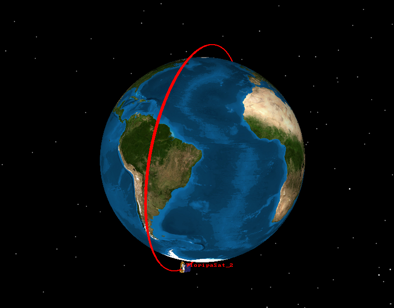
Fig. 5 GOLDS-UFSC orbit simulation on GMAT.
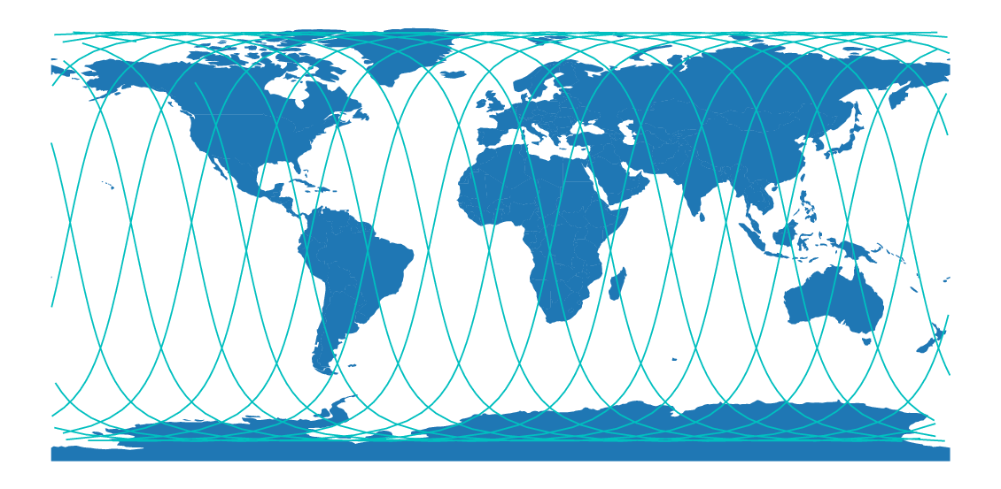
Fig. 6 GOLDS-UFSC simulated groundtrack.
The next sections present some analysis based on the results obtained from the simulations performed with SimCube.
Lifetime Analysis
Considering the same parameters of FloripaSat-1, but with an initial altitude of 550 km, the simulations on SimCube showed that the satellite decays approximately in 2183 days (\(\cong\) 6 years), as can be seen in Fig. 7.
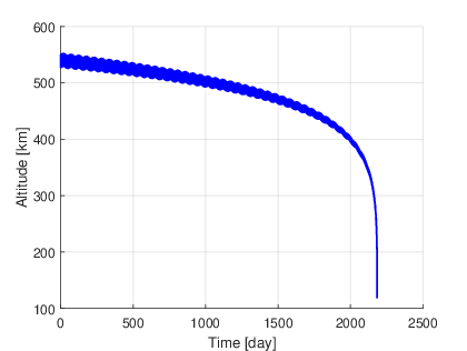
Fig. 7 Lifetime analysis.
Ground Station Passes and Data Transfer Analysis
Considering two ground stations, one at the SpaceLab installations in Florianópolis (27° 36’ 00.9” S, 48° 31’ 03.2” W) and other at the INPE/CRN installations in Natal (5° 50’ 10.1” S, 35° 12’ 27.5” W), both with a minimum elevation of 15°, the results in Table 7) were achieved.
Parameter |
UFSC Station |
INPE-RN Station |
Unit |
|---|---|---|---|
Minimum elevation to a valid contact |
15 |
15 |
° |
Number of contacts |
143 |
125 |
|
Minimum contract period |
24 |
34 |
sec |
Maximum contact period |
395 |
394 |
sec |
Average contact period |
303 |
298 |
sec |
Total contact period |
43394 |
37205 |
sec |
As seen from Table 7, during the first 60 days of operation, considering the two main ground stations that will contact the satellite, the total contact period is 80599 seconds (43394 + 37205). With the data rate of the downlink/uplink as 4800 bps, this period will allow a data transfer of 48359400 bytes (or 46.12 MiB) between GOLDS-UFSC and the Earth. Using the satellite’s lifetime from the previous analysis (2000 days), and an average data transfer per day of 805990 bits, the total theoretical raw data transfer during the whole operation of the satellite will be approximately 1.5 GiB.
These values can be even more significant if a smaller minimum elevation is considered, or with more ground stations in other locations.
Mass Budget
The mass budget of the satellite can be seen in Table 8.
Subsystem |
Model |
Mass [g] |
|---|---|---|
OBDH |
SpaceLab OBDH 2.0 |
53 |
TTC |
SpaceLab TTC 2.0 |
52 |
EPS |
SpaceLab EPS 2.0 |
80 |
Battery |
SpaceLab Battery Module 4C |
235 |
Antenna |
ISISpace AntS |
89 |
ACS |
SpaceLab Passive ACS 2U |
100 (TBC) |
Payload |
INPE-RN EDC |
75 (×2) |
Radiation instrument |
SpaceLab Payload X |
75 (TBC) |
Interface |
SpaceLab Interface Boards |
40 |
PC-104 Adapter |
SpaceLab PC-104 Adapter |
50 (TBC) |
Solar Panel |
Orbital Custom Solar Panel |
266 |
Shields |
3 mm aluminum sheets |
590 (TBC) |
Structure |
Usiped Custom 2U Structure |
206 |
Cables |
200 |
|
Others |
100 |
|
Total |
2211 |
|
Max. CubeSat 2U |
2666 |
|
Margin |
455 |
According to the CubeSat standard [40], the maximum mass of each unit must be 1.33 kg. As the GOLDS-UFSC is a 2U CubeSat, the maximum allowed mass of the project is 2.66 kg. Considering the weight of each subsystem presented in Table 8, the current total mass of the object is below the maximum allowed, with a margin of 16 %.
Power Budget
According to section 10.3 of [33], the power budget of a satellite can be determined through three steps:
Prepare operating power budget
Size the battery
Estimate power degradation over mission life
Input Power
Simulations of the energy input to the solar panels along some orbits can be seen in the Fig. 8 graph. Two extreme orbit scenarios, without and with maximum eclipse, were tested. The figures show the power generated on each side of the CubeSat, as well the total and average values.
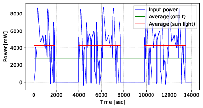
Fig. 8 Simulated input power of the solar panels.
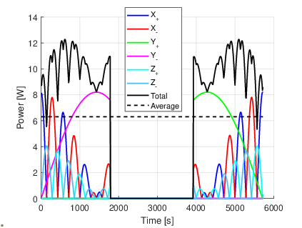
Fig. 9 Maximum eclipse.
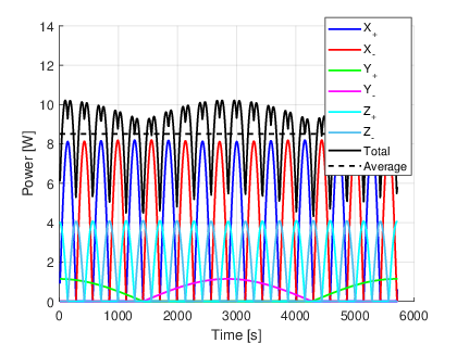
Fig. 10 Without eclipse.
From these simulations, the results in Table 9 were obtained:
Parameter |
Maximum eclipse |
Without eclipse |
|---|---|---|
Peak power |
12282.7 mW |
10217.2 mW |
Average power (total orbit) |
6306.9 mW |
8519.6 mW |
Average (sunlight) |
10048.9 mW |
8519.6 mW |
Orbit period |
5720 s |
5720 s |
Sun light period |
3590 s |
5720 s |
Eclipse period |
2130 s |
0 s |
Operating Power Budget
Typical operating voltages and current and power ranges consumed by each satellite subsystem are presented in Table 10.
Module |
Voltage [V] |
Current min. [mA] |
Current max. [mA] |
Power min. [mW] |
Power max. [mW] |
|---|---|---|---|---|---|
OBDH |
3.3 |
35 |
200 |
115 |
660 |
TTC (µC) |
3.3 |
40 |
40 |
132 |
132 |
TTC (radio module) |
5 |
10 |
650 |
33 |
3250 |
EPS (digital part) |
7.4 |
50 |
260 |
165 |
858 |
EPS (heater) |
7.4 |
675 |
675 |
5000 |
5000 |
Antenna module |
3.3 |
60 |
550 |
200 |
1800 |
Payload EDC |
5 |
250 |
250 |
1250 |
1250 |
Radiation instrument |
5 |
TBD |
TBD |
TBD |
TBD |
Using the information presented in Table 10, and the activation periods defined for each module (the duty cycle), we arrive at the average satellite consumption present in Table 11.
Module |
Duty Cycle [%] |
Power [mW] |
|---|---|---|
OBDH |
100 |
115 |
TTC (radio 1 RX) |
95 |
65 |
TTC (radio 1 TX) |
5 |
3250 |
TTC (radio 2 RX) |
95 |
65 |
TTC (radio 2 TX) |
5 |
3250 |
EPS |
100 |
320 |
BAT (idle) |
90 |
0 |
BAT (heater full) |
10 |
5000 |
Antenna (deployment) |
0 |
1800 |
Antenna (deployed) |
100 |
35 |
Payload EDC |
100 |
1250 |
Radiation instrument |
0 |
1000 |
Satellite |
\(\cong\) 2668 |
The duty cycles of Table 11 were defined according to the following assumptions:
One of the EDC payload is always off (cold redundancy).
The Radiation instrument is turned on just during limited periods and only with telecommands.
As can be seen from Fig. 8 and Table 11, there is a slight positive margin of 76.9 mW in the power budget.
Battery Sizing
As described in [33], the battery sizing of a satellite can be made by following the steps below:
Estimate power level that the battery must supply
Compute discharge cycle duration, charge cycle duration, and numbers of charge-discharge cycles
Select depth of discharge
Select charge rate
Compute battery recharge power
The power level that the battery must supply is the total power consumption of the satellite and is available in Table 11.
The discharge and charge cycle duration can be obtained from Fig. 8. The discharge duration is approximately 35.3 min (or 0.5889 h), and the charge cycle duration is 61.83 min (or 1.031 h). This is considering a single complete orbit.
The depth of discharge (DoD (Depth of Discharge)) can be obtained using the (1).
Where:
\(D_{i}\): Discharge rate
\(D_{t}\): Discharge period
\(C\): Battery capacity
As the battery cells are already selected (5000 mAh in total, as described in Battery Module), the current DoD is computed in (2).
The charge rate can be estimated from the power input of the solar panels when the satellite is in sunlight. As presented before, the simulation results estimate the power input as 4315.6 mW. Considering the charge time as 61.83 min (or 1.031 h), the input energy is 4450 mWh. From Table 11, the power consumption of the satellite at sunlight is 2169 mW (or 2236 mWh considering the sunlight period). This way, energy input at sunlight is obtained in (3).
From the DoD calculation, the energy consumption during the eclipse is 1571 mWh. This way, the energy margin of the battery becomes positive (\(2214 - 1571 = 643 mWh\)), as expected from the power budget results.
All results from the battery sizing are available in Table 12.
Parameter |
Value |
Unit |
|---|---|---|
Battery capacity |
18500 |
mWh |
Energy consumption on sunlight |
2169 |
mWh |
Energy consumption on eclipse |
1571 |
mWh |
Sunlight duration |
1.031 |
h |
Eclipse duration |
0.5889 |
h |
Depth of Discharge (DoD) |
8.5 |
% |
Total battery energy margin |
643 |
mWh |
From the results, the battery sizing is well suited for the current satellite configuration and the planned behavior.
Power Degradation Over Mission Life
Two major events along the satellite operation should be considered in the power degradation analysis:
Solar panels degradation
Battery degradation
From [33], 5 % per year is a usual number for the solar panels’ degradation, in other words, the general efficiency of the solar panels decays at a rate of 5 % per year of operation.
Link Budget
The link budget of all satellite radio links is available in Table 13.
Variable |
Beacon |
Downlink |
Uplink |
Uplink (Payload) |
Unit |
|---|---|---|---|---|---|
Altitude |
550 |
550 |
550 |
550 |
km |
Elevation |
0 |
0 |
0 |
0 |
° |
Frequency |
146 |
450 |
450 |
401.635 |
MHz |
Modulation |
GMSK |
GMSK |
GMSK |
BPSK |
|
Protocol |
NGHam |
NGHam |
NGHam |
SBCD |
|
Transmit power |
30 |
30 |
44 |
30 |
dBm |
Transmitter antenna gain |
0 |
0 |
12 |
3 |
dBi |
Receiver antenna gain |
12 |
12 |
0 |
0 |
dBi |
FSPL |
144.4 |
154.2 |
154.2 |
153.2 |
dB |
Power at receiver |
-107.4 |
-117.2 |
-103.16 |
-125.2 |
dBm |
Receiver sensibility |
-134 |
-134 |
-126 |
-128 |
dBm |
System losses |
5 |
5 |
5 |
5 |
dB |
Receiver noise temp. |
361.7 |
361.7 |
361.7 |
361.7 |
K |
Antenna noise temp. |
300 |
300 |
300 |
300 |
K |
System noise temp. |
661.7 |
661.7 |
661.7 |
661.7 |
K |
Data rate |
1200 |
9600 |
9600 |
400 |
bps |
Received SNR |
32.22 |
13.41 |
27.41 |
19.17 |
dB |
SNR required for \(10^{-5}\) BER [1] |
9.6 |
9.6 |
9.6 |
9.6 |
dB |
Link margin |
\(\geq\) 22.62 |
\(\geq\) 3.812 |
\(\geq\) 17.81 |
\(\geq\) 9.57 |
dB |
As can be seen, considering the worst case for the estimated orbit, that is, with the satellite on the horizon and with an elevation of zero degrees, the margin of all links is positive with a considerable balance.
All equations and steps used to obtain the results of Table 13 are available in Link Budget Calculation.